Field Trials of AML Instruments - Surveying the Squamish Inlet
With John Hughes-Clarke from the Ocean Mapping Group of UNB
By: Ian Lougheed, B.Eng, EIT Mechanical Engineer - AML Oceanographic
Introduction
AML Oceanographic had a unique opportunity in July 2012 to test and use their instruments as part of field research by renowned researcher John Hughes-Clarke. John Hughes-Clarke is a Professor and Chair of Ocean Mapping at the University of New Brunswick (Canada). His research areas include studies on spatial resolution of multibeam sonar systems, remote seabed characterization, and seabed formations generated by sediment transport. John is known for his detailed work, excellent presentations, and aggressive use of the MVP30 system. The MVP30 system uses the AML Micro CTD or Micro SVTP instrument mounted on the back of a fish.
Background: The Canadian Hydrographic Conference - May 2012
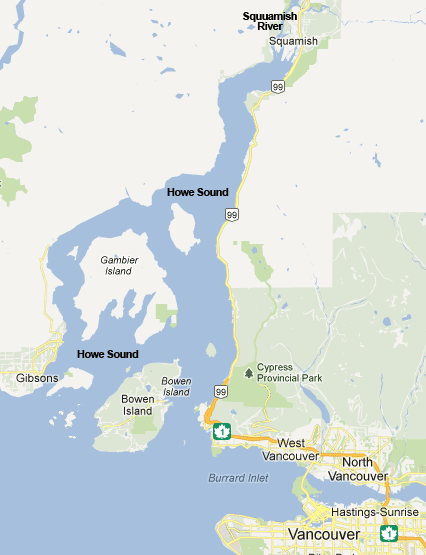
John presented at the The Canadian Hydrographic Conference in May at Niagara Falls, Ontario, Canada, which AML Oceanographic attended. His presentation focused on his team’s ongoing research regarding the Squamish Delta in Howe Sound, near Vancouver, British Columbia, Canada.
The Squamish River discharges into Howe Sound, creating the Squamish Delta. The river and delta were narrowed during 1971 to install a training dyke to make room for a harbour. This narrowing made the river run deeper and faster into the delta, causing substantially increased suspended sediment transport. This sediment is continually deposited in the delta, causing it to advance and change shape rapidly (approximately 4 meters per year). In this portion of the delta, the depth ranges from 3-4m right at the river exit to over 200m at the southern end of the delta. As this prodelta (submerged delta) changes, it is closing off the harbour. His presentation showed very detailed time-lapse images of the Squamish Delta seabed. He discussed the mechanisms of growth of the sediment deposits and how this leads to underwater landslide events. These landslide events are triggered by many factors including tidal cycles and trapped gas deposits. John’s ongoing research contributes to many facets of oceanography, from accuracy of navigation and sonar imaging to the design of engineered landscapes and
slopes. At the Conference, Ian Lougheed, a Mechanical Engineer with AML Oceanographic approached John to see if we could participate in this research and provide assistance. John welcomed AML to collaborate, and here we discuss the initial results from these efforts.
Vessel and Equipment
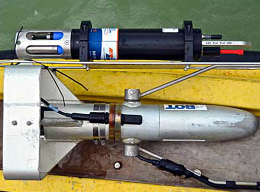
The Heron is a 10 metre research vessel owned by the Ocean Mapping Group of UNB (OMG). On its hull is a Kongsberg EM-710 multibeam SONAR transducer, with the AML Micro SV instruments next to it for surface sound speed. On the back of the Heron is the MVP-30 system. The MVP-30 is the smallest of the Moving Vessel Profiler systems. The fish is small, and fits a right-angled AML Micro CTD instrument in its body. Two OBS (turbidity) sensors are connected to the AML Micro instrument through analog channels. The following picture shows the overall system. The winch is in blue, underneath the step. The pulley and guide system on top contains some cable payout monitoring, as well as heavy duty guides for controlling cable payout and recovery. For more information on the Heron vessel, visit UNB's website here.
AML Products Used in Research
AML Instruments:
Minos·X
Micro SV
Micro CTD (deployed via MVP-30)
Xchange™ Sensors:
SV·Xchange™ (Sound Velocity)
P·Xchange™ (Pressure)
T·Xchange™ (Temperature)
Turbidity·Xchange™
AML Oceanographic Engineers:
Ian Lougheed, B.Eng, EIT Mechanical Engineer
Dustin Olender, PhD, EIT Mechanical Engineer
Field Research
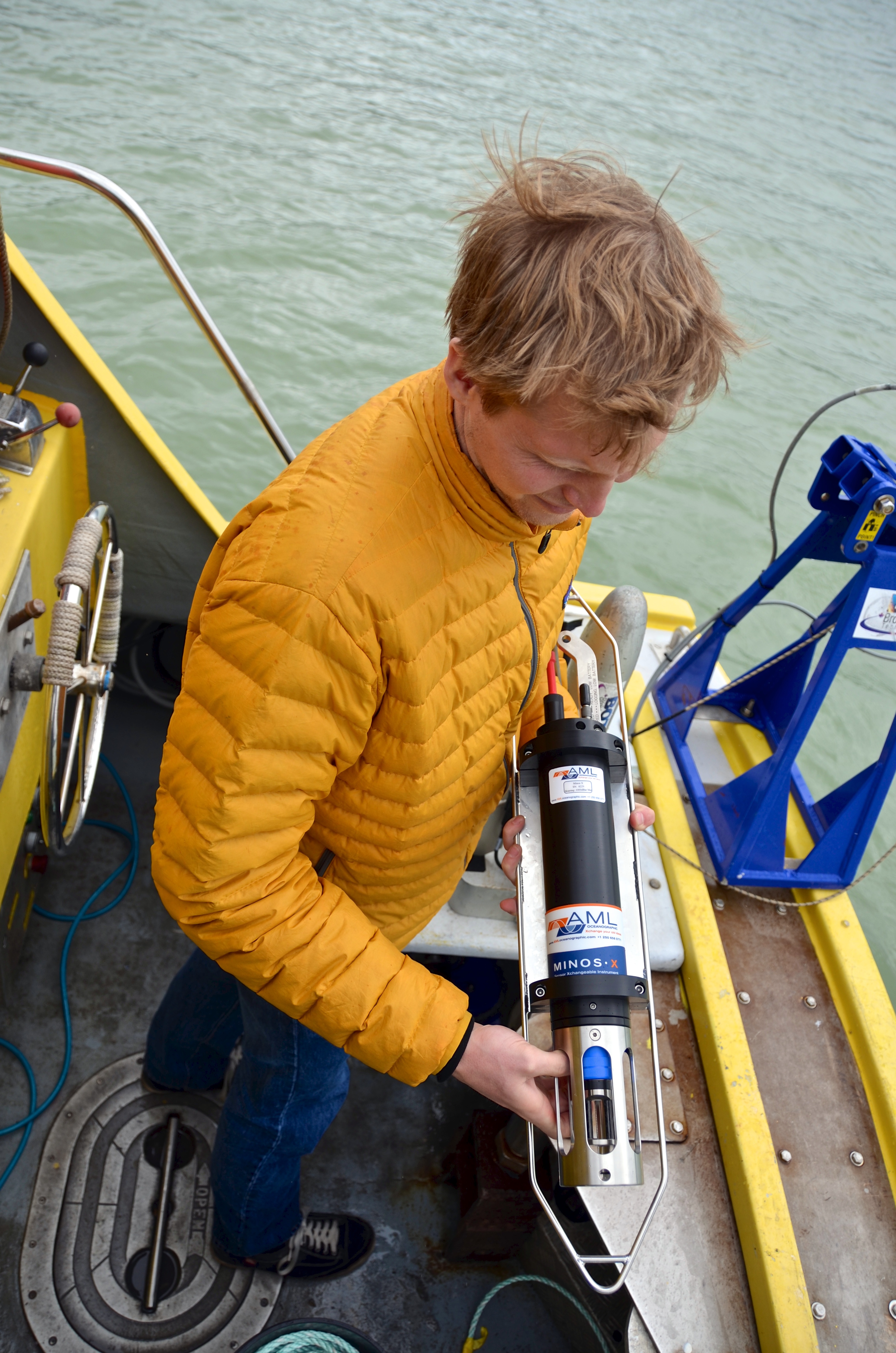
Each day of research involves constantly running the MVP system while collecting numerous overlapping multibeam images of the sea bed. The MVP is used to collect sound speed profiles (calculated, since it’s a CTD), as well as turbidity profiles with two turbidity sensors. This is where AML’s prototypes could be of service. Shown at right is Dustin Olender, Ph.D., Mechanical Engineer with AML’s Minos•X.
With all of this information, John documents accumulation of sediment structures during high tide, and their potential collapse at low tide. His turbidity sensors provide him with a measure of sediment outflow from the river, and the multibeam images can resolve very subtle changes in the shape and size of the delta.
One of the most surprising things we learned is that John can actually “see” sediment clouds with his multibeam system. Using the backscatter (echo) data, and his own self-written software, he can visualize plumes of sediment above the sea bed. This is possible because sediment reflects a small amount of acoustic data before the main reflection comes from the sea bed. He also pointed out plumes of gas discharge and clouds of plankton that we could also see using the same principle. This is an amazing and uncommon use of multibeam data.
In total, John collects several hundred MVP profiles per day, and dozens of passes worth of multibeam images of the delta. For this reason, John’s research is a very aggressive test bed for the MVP system. In contrast, many commercial hydrographers will collect between 2 and 5 MVP profiles per day, depending on conditions. Even though the MVP system is automated, surveyors only require that many profiles to reach current standards of multibeam data accuracy.
The Data
We collected a significant amount of data with Minos•X alongside the Micro CTD. There were seven comparative casts taken throughout the day. Most of these had Minos•X configured with Sound Velocity, Pressure, and Turbidity Xchange™ sensors. This configuration allowed us to compare Sound Velocity and Turbidity profiles with the Micro CTD. One cast was taken with Temperature in place of Turbidity, allowing us to calculate Salinity from our Sound Velocity profile and compare that to Salinity from the Micro CTD. Only X-Series instruments with Xchange Field-swappable sensors provide this level of configurability in the field.
Sound Velocity Casts
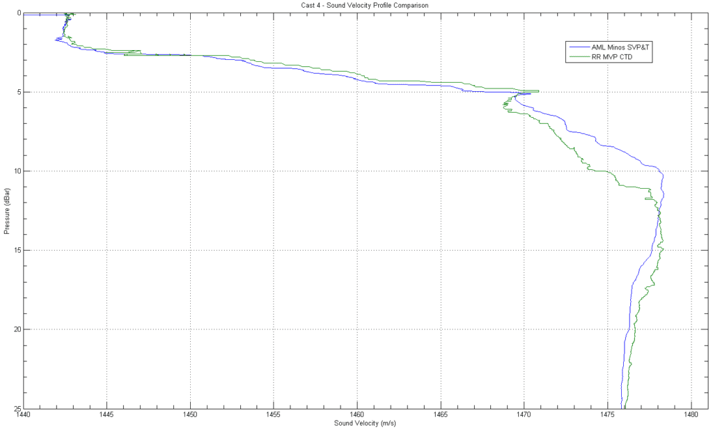
The first plots to discuss are from the fourth cast we performed. In this cast, Minos (with SV,T, and P Xchange™ sensors) was tied to the MVP fish, with sensors aligned. A picture of the setup is shown at right.
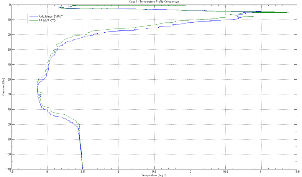
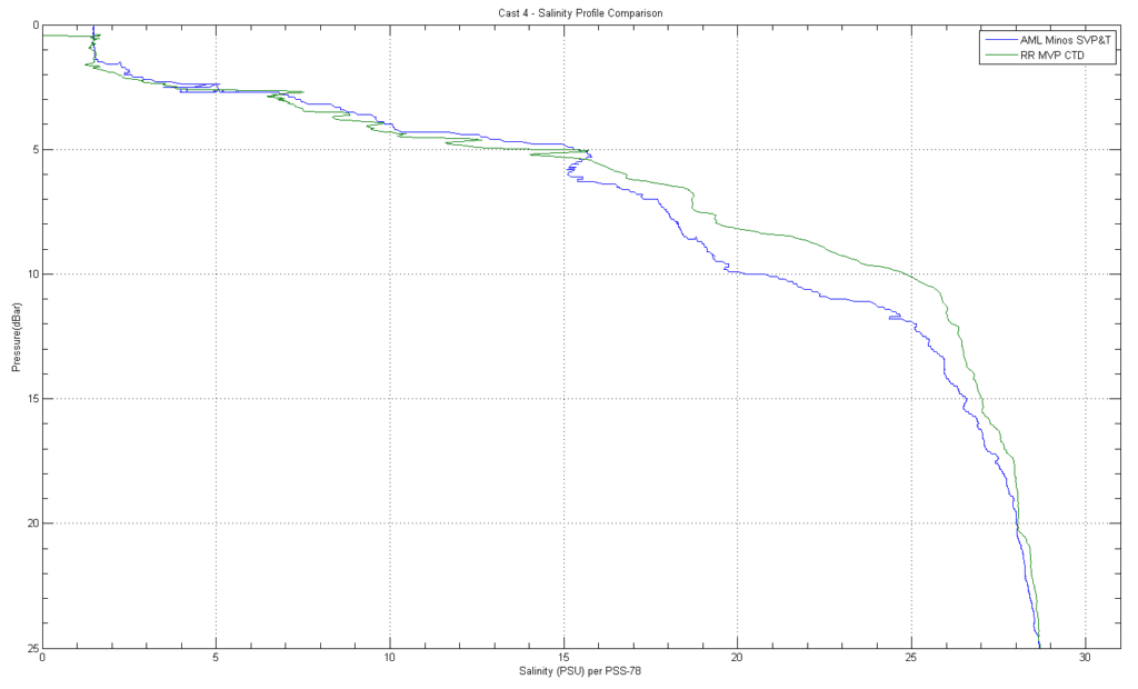
Both the MVP towfish and Minos•X were lowered to 120m using manual control of the MVP winch. There are some interesting features of this profile. In the top 2m of water, we see a sound speed around 1443m/s. This is the fresh, cool water coming out of the river and stratifying to the top. A glance at the temperature and salinity plots below will show this cool, freshwater layer at the top. Since this top layer is fresh, it is less dense than the salty ocean water in the delta, so it tends to stay on top (stratify) until mixing occurs.
From 2m to 10m we observe a very rapid shift in sound speed up to about 1478m/s. This transition is shaped both by the rapid change in salinity (see the third plot), and some of the wild fluctuations in temperature. This is the type of situation where “Salinity spiking” from a CTD can cause significant errors when calculating sound velocity, while AML’s time-of-flight SV sensor is capable of resolving these fine details of the profile without introducing errors. You can observe some of these differences in the sound velocity profile, where variations of 3-4m/s can be seen between 5 and 20m depth. This isn’t a pressure sensor offset (they line up perfectly at the 2-3m depths). It’s a fundamental difference between calculated SV and directly measured SV.
We also observe error between calculated and measured sound velocity due to an inherent assumption in the CTD to SV calculation. Different salts are assumed to be in a particular ratio, specifically the same ratio as the water used in the original UNESCO Equation of State of Seawater research. In a Pacific Northwest river delta, it is unlikely that salts are dissolved in the same ratios as those found mid-Atlantic. Thus, different salinities can create the same conductivity for a sensor. Time-of-flight sound velocimetry removes the question of salt ratios entirely, focusing on the end-game: speed of sound.
Finally, be aware that these two instruments are measuring slightly different water spatially. Even though they’re close together, there will be local variations that can account for some of the measured differences.
Cast 4 - Temperature Profile (Note the scale, this goes to the full 110 depth)
Cast 4 - Salinity Profile from 0 25m
Turbidity Profiles and Measurements
A key area of John Hughes-Clarke’s research is turbidity measurement. He uses turbidity profiles to validate his sediment plumes as visualized by his multibeam system. With these turbidity measurements, he can detect underwater landslide events, gas vents, and other details that may otherwise go undocumented with pure multibeam data. He is using two turbidity sensors as analog channels on his MVP fish. However, they aren’t calibrated with respect to sediment concentrations. All he can visualize is relative changes in turbidity.
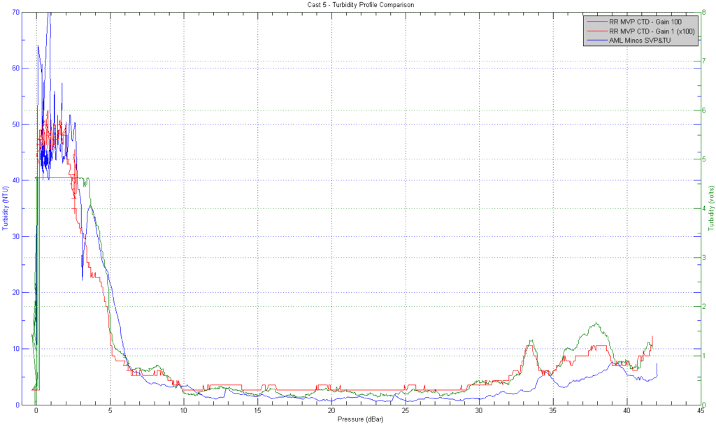
A note about John’s 2 turbidity sensors. He found his original turbidity sensor was not sensitive enough for some less turbid water. He ordered a second unit with a gain of 100x applied, making it 100 times more sensitive. In tandem, he can measure a fairly wide range of turbidities. However, when the water gets quite turbid, the 100x gain unit saturates at about 4.6 volts. For the plots below, I’ve multiplied the unity gain sensor output by 100 so its values are comparable to the 100x gain sensor on the same set of axes.
We brought some of the new AML’s Turbidity•Xchange™ sensors, which are actually calibrated with respect to the Nephelometric Turbidity Unit (NTU). These give an absolute measurement of turbidity than can more easily be related to sediment concentration.
We took about 6 comparative turbidity profiles. Our 5th cast is shown below, to give a sense of what we were working with. The top 2-3m is highly turbid (from 40-80 NTU). This is the stratified layer of dirty, sediment-filled river water. The sediment levels quickly drop off as we enter the cleaner, saline ocean water. However, near the bottom, turbidity levels begin to peak again. These are the features John is looking for, as they are plumes of sediment that are carried up and down the delta sea bed by complex currents.
Performance of AML's Turbidity·Xchange™ Sensor
In the highly turbid water (top 3m), John’s 100x gain turbidity sensor (the green line) saturates. However, even at this scale, the unity gain sensor (red line) provides very coarse readings. You can see the step size between samples. This is a low-resolution solution. In comparison, the resolution of Turbidity•Xchange™ is vastly greater. Turbidity•Xchange™ isn’t resolution limited, even though it is operating in less than 1/10th of its total range (0- 1000 NTU!). This is impressive!
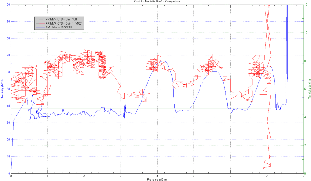
To further highlight the performance of AML’s Turbidity•Xchange™ sensor, I’d like to look at another plot below. Here, we did a dip right in the river until we hit the bottom about 7m deep. We took a bottle sample of the water which John is going to have tested for particle concentration. Since this was very turbid water, the 100x gain sensor (Green) saturated the whole time. However, there are two interesting comparisons to draw between Hughes-Clarks’s unity gain turbidity probe and Turbidity•Xchange™.
- First, look at how coarse the samples are along the red curve. It appears to be jumping all over the place, even backwards sometimes. In the vertical direction, you’re again seeing the resolution limit of these sensors. This is the actual step size of the analog to digital and digital to analog conversion. And, at any particular depth, you can expect a few “counts” or steps of noise in the data. During this deployment, we stopped lowering the instruments at a couple of points. On the red curve, you can see a few places where a cloud of points bounces left and right in a vertical line. That is noise! AML’s sensor, however, still has no visible steps. Our sensor was stopped at the same times, and maintains very consistent readings (not bouncing up and down). AML’s resolution is far superior, even though we’re operating within 1/10th of our total range! The detail we can resolve, and the repeatability of our readings are really impressive.
- The second point I’d like to illustrate is based on how the sensors work. Now, I’ve “visually calibrated” the analog sensors to our turbidity sensor by matching up the curves. But, from about 0-3 meters depth, the red line (theirs) and the blue line (ours) don’t match up at all. Remember that John’s turbidity probes are Optical Backscatter types (OBS). AML’s is Nephelometric. OBS sensors are typically sensitive to ambient light, since they rely on “mirror-style” reflection of light. Nephelometric sensors rely on a 90-degree measurement, and are much less sensitive to ambient light. I believe what we see from 0-3 meters is actually the difference in ambient light sensitivity. Below 3m, little of the daylight penetrates the water, and the readings correlate more closely. Another testament that we’re on the right track with our Turbidity•Xchange™ sensor.
Learn how MVP can make a difference for you.
AML’s Moving Vessel Profiler is proven to remove both the technical and financial unpredictability associated with survey operations. With over 130 systems sold, MVP is the market leader in underway profiling systems, and is backed by 20 years of experience and thousands of successful surveys.