Accuracy Is a Choice: Profiling Frequency and Managing Sound Velocity Error

A conversation with industry expert Jonathan Beaudoin

Accuracy is a choice. In everyday field operations, your sound velocity cast starts aging the moment you collect it. 
Ideally, the ocean would be uniform from top to bottom, but that is almost never the case. In the most complex conditions, oceanography can change minute by minute - a cast from 15 minutes ago may be outdated.

The right frequency isn't a fixed number, it's a judgment call driven by how fast the ocean around you is changing. This piece walks through why that's true, and what it looks like in practice.

Sound Velocity (SV) and Survey Accuracy

Sound waves don't travel in a straight line underwater. They refract through layers of varying temperature and salinity often creating two problems at once. Refraction distorts where surveyors think the beam landed, and scaling distorts how far it travelled along the ray path. “Smiles” and “frowns” will appear as the edges of the swath curve up or down. These patterns are a clear red flag that the seafloor is being mapped inaccurately, often leading to rework and safety risk. If the sound velocity (SV) profile is outdated, too sparse, or miscalibrated, depth and location are both compromised. Consequences of this bias are repeatable and systematic: surveyors say “garbage in, garbage out”. No amount of post processing can fully fix a warped data set. 

Episode one: “Smiles, Frowns & Misplaced Seafloors: The Case for Accurate Sound Velocity Data” made it clear: when SV is wrong, your entire survey may look perfect, while being fundamentally biased. This is exactly why frequency deserves more attention than a simple, fixed interval gives it. If clean data can still be wrong, the real question isn't whether your survey looks good, it's whether you profiled often enough to catch dynamic ocean conditions as they change.

When Precise Data Is Still Wrong

Precise doesn’t mean accurate. A survey can appear internally consistent - smooth and repeatable - while still carrying residual bias if sound velocity conditions are not fully captured. 

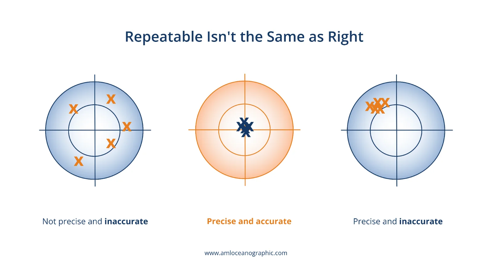
Precision alone doesn't guarantee accuracy.

Post-correction, the gridded bathymetry may appear smooth, with reduced distortions and acceptable statistical metrics. But smiles and frowns are the visible symptom of undersampling - and processing away the symptom doesn’t correct that underlying gap in coverage. The data may look improved - but is still not fully representative of the true seafloor. 

In this context, precision means the data agrees with itself, achievable in a single survey pass, since there is nothing yet to compare it against. Repeatability only gets tested with a second, independent pass of the same area. It’s entirely possible for this pass to be just as precise on its own, and still not line up with the first. Two passes only agree when the sound velocity behind them is accurate, assuming all other sources of error and bias are well managed. That's the target: not precision, but accuracy. And profiling frequency is what gets you there.

Much of this thinking is explored in more depth in Jonathan Beaudoin’s Multibeam Crash Course.

Choosing the Right Profiling Frequency

If the cost of outdated SV is significant bias, rework and safety risk, then profiling frequency becomes one of the most important decisions you make. So how often is enough?

While it’s a popular default, you likely need to do more than 1 cast every 2 hours. Profiling frequency should be driven by ocean variability, not just the clock. If sound velocity changes faster than profiles are collected, bias can quietly accumulate and persist for long periods before it’s detected. 

This creates a fundamental tradeoff. More time profiling improves accuracy, but traditional casting methods introduce downtime and increase operational costs. If no downtime or budget increases were involved, surveyors would profile infinitely. In reality, every cast competes with productivity. 

This is where the idea of a “Goldilocks” frequency applies. Too few profiles, and you risk systematic bias. Profile too often, and efficiency suffers. Better, is somewhere in between - a frequency that reflects actual environmental variability rather than arbitrary time intervals.

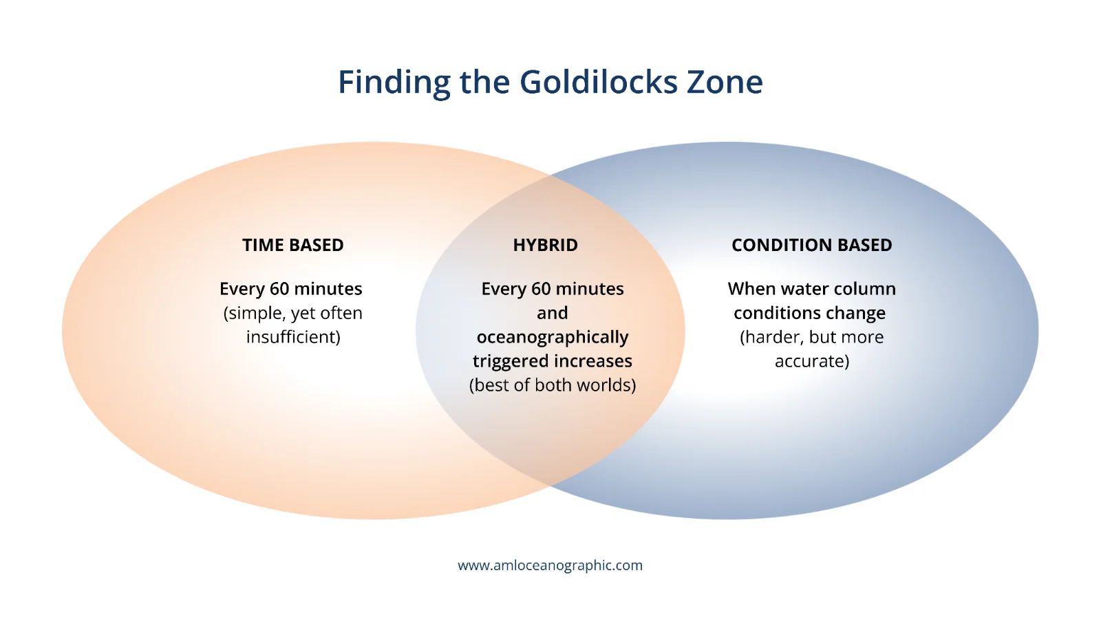
The hybrid approach: a fixed baseline, adjusted upward when oceanographic conditions change.

While the hybrid approach is more effective than time or condition based triggers alone, this is a guide, not a guarantee, and it still assumes every additional cast costs time and money. Underway profiling systems change the conversation entirely: they remove this assumption. By reducing downtime and therefore operational costs, tools like the Moving Vessel Profiler (MVP) improve accuracy without sacrificing efficiency. It’s no longer a careful balance, surveyors can have both: sample continuously underway with impunity. 

The Hydrographer Mindset

In practice, client specifications for minimum SV sampling intervals are often not sufficient to achieve the level of accuracy being demanded. For example, an end client may specify a minimum sampling interval - say, four casts per day. But hydrographers shouldn’t fall into the trap of treating that as adequate. The client doesn’t see what you see in the field, and it’s ultimately your responsibility to ensure the required accuracy is achieved. This can mean taking more casts than originally specified. 

As oceanographic experts, the onus is on the hydrographers to over deliver on the SV spec in order to achieve the required accuracy. Study oceanography and employ your intuition. 

While oceanographic models may help hydrographers anticipate variability, one of the most valuable opportunities during data acquisition is the ability to observe conditions in real time. Keeping systems active and reviewing incoming data allows surveyors to spot patterns early - often through visual clues alone. Subtle inconsistencies, minor changes in surface sound speed behavior, or features that just “don’t quite seem right”, are often early indicators of sound velocity issues. 

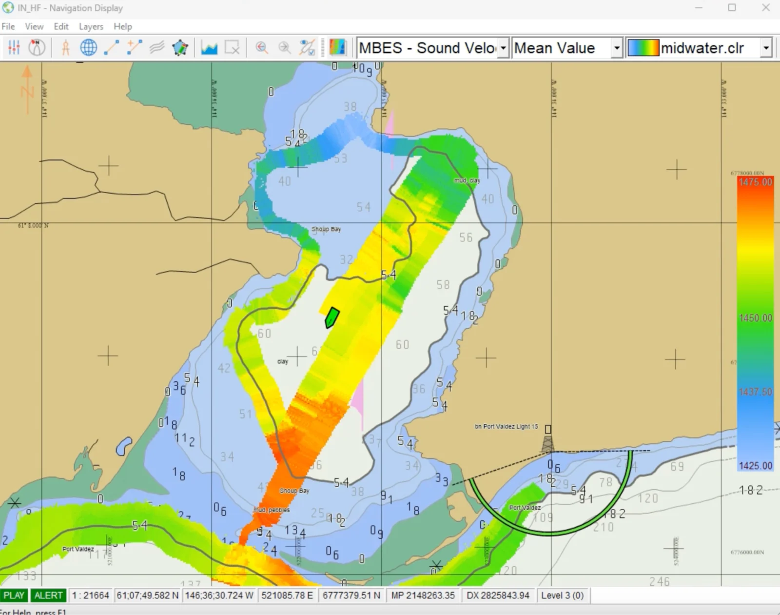
An example of a real-time map of surface sound speed, as read by the sound velocity sensor at the transducer. This map was created using QPS Qinsy 9.8.0. Maps like this provide a clear view of spatial patterns and help identify areas that may require closer attention.

A practical example of a period where sound speed structure changes significantly is local solar noon. During periods of peak solar heating, near-surface sound velocity can change more rapidly. As a result, profiles age faster than at other times of day, and the sampling rate may need to be increased. This is what "driven by ocean variability, not the clock" actually looks like day to day: recognizing when conditions are actively evolving, and responding accordingly, rather than relying on the clock alone.

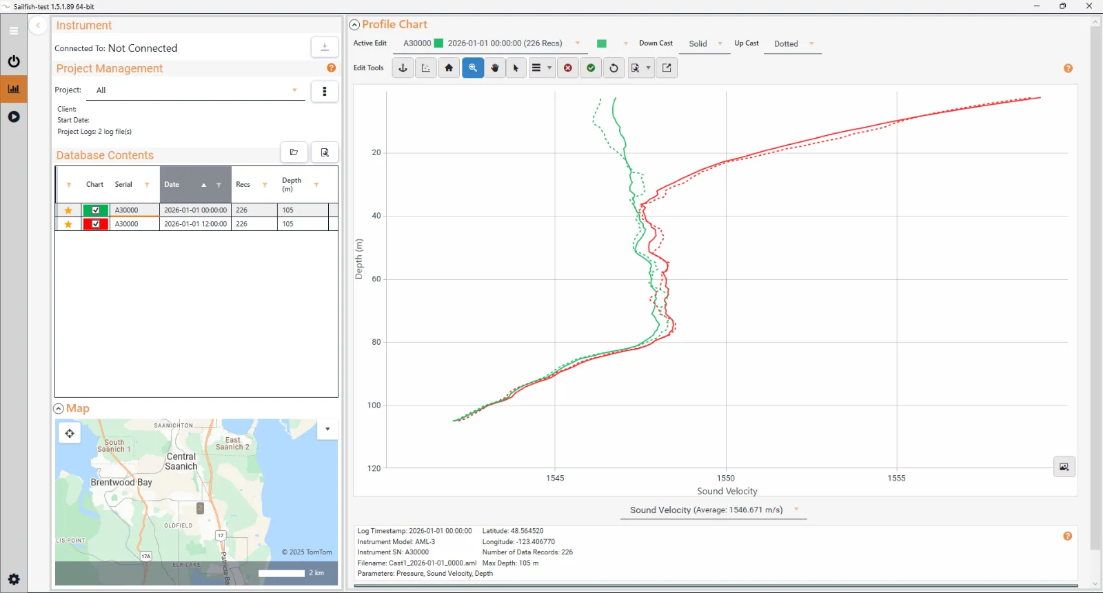
Illustrative example from Sailfish: two casts, same site, 12 hours apart. Below ~40m, the profiles match closely. Near the surface, they diverge, consistent with solar heating over the course of a day. A morning cast may not reflect afternoon conditions near the surface, even when deeper water hasn't changed.

There's also a more quantitative way to make this same judgment, developed by Jonathan alongside NOAA and Woolpert: calculate the harmonic sound speed of each cast, then compare it to the previous one. A big difference means it's time to profile more. This isn't theoretical. NOAA's experimental Moby Sound Speed TPU Estimator applies exactly this concept in the field. Survey teams using it have adjusted their casting interval accordingly, in one case relaxing from every 2 hours to every 4.

How much margin for error you have will shape how closely you need to track that variability. High risk operations, say, concerning safety of navigation, leave less room to fall behind the ocean's changes than a lower stakes mission like a quick localization job. Different applications may justify different cast frequencies. That said, no client complains about good data - there is no practical upper limit on accuracy.

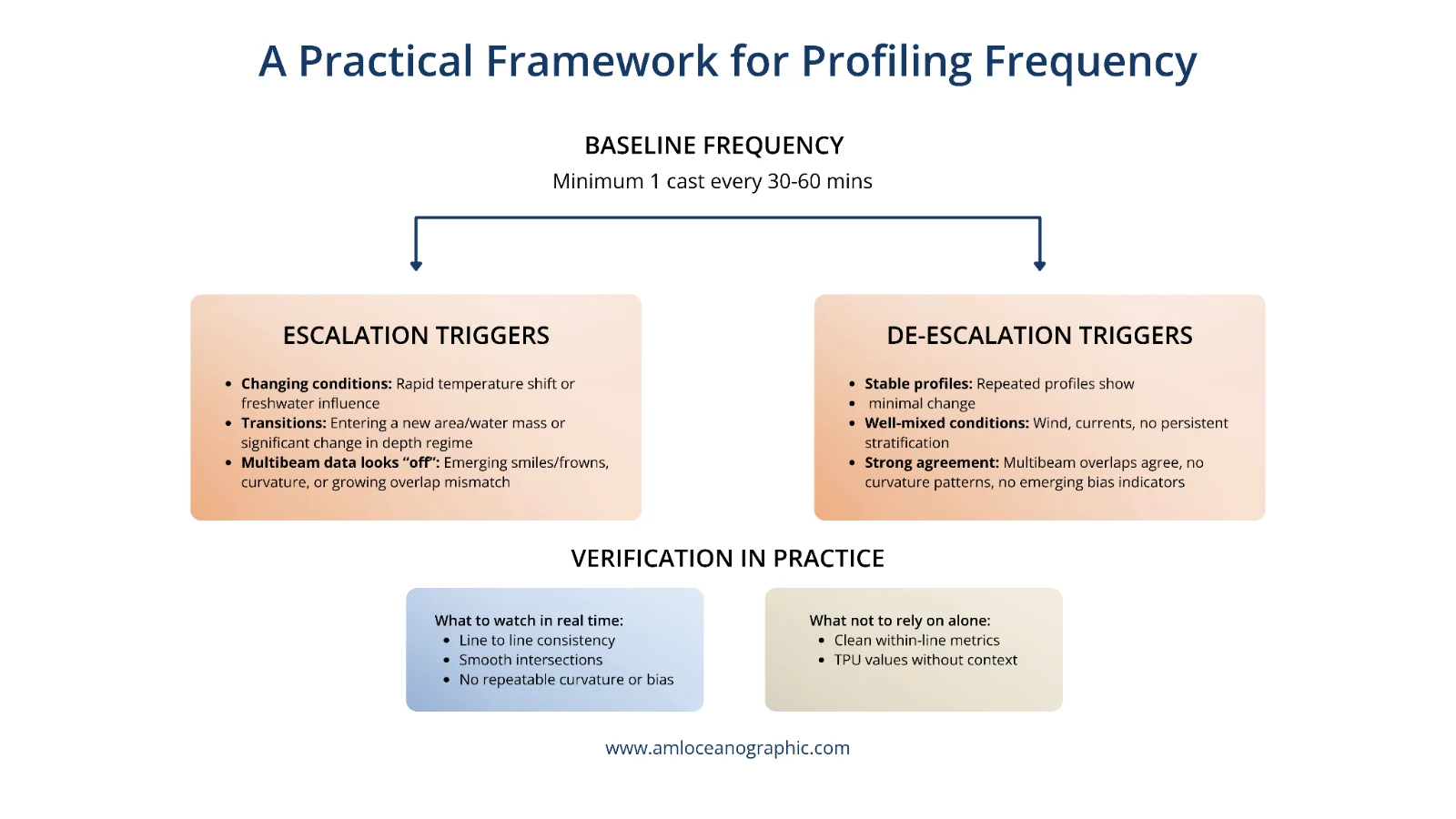
The hybrid approach as a working decision framework. 

Sound velocity errors are often visible in real time through artifacts and inconsistencies in the data. The challenge lies in interpreting and resolving those signals correctly. If profiling is too infrequent, or environmental changes are not fully captured, bias can persist even after visible issues have been addressed. Put simply, it isn’t about meeting a minimum requirement or following the clock; it’s about keeping pace with a dynamic ocean. 

Profiling frequency is the primary control surveyors have to manage this risk - a practical expression of choosing accuracy over convenience. 

This article is part of an ongoing series of discussions with Jonathan Beaudoin of HydroOctave Consulting, whose work in multibeam sonar informs much of the conversation.